
Python for Financial Analysis: A Stock vs SPY in pandas
Python for financial analysis starts with daily closing prices and a few pandas operations. pct_change gives daily returns, a compounded ratio gives CAGR, and the daily standard deviation times the square root of 252 gives volatility. cummax finds drawdowns, and covariance over variance gives beta. This post runs each on NVDA against SPY over five years.
Every code block on this page was run on November 4, 2026 with Python 3.13.8, pandas 3.1.0, NumPy 2.5.4, yfinance 1.8.0 and matplotlib 3.11.2, in the order shown. Each output is pasted from that run. Prices are daily closes from Yahoo Finance via yfinance (unofficial), November 1, 2021 to October 30, 2026; Yahoo’s data is covered by its terms of service. NVDA is an example, not a recommendation, and past returns don’t predict future ones.
Key takeaways
yf.downloadadjusts prices for dividends by default (auto_adjust=True) and drops the Adj Close column, so older code that reads["Adj Close"]raises a KeyError.- Over these five years NVDA returned 695.8% (51.5% a year) with 51.9% annual volatility. SPY returned 75.6% (11.9% a year) with 17.2%.
- NVDA’s maximum drawdown was -66.3%, from November 2021 to October 2022, and it didn’t close back at that high until May 25, 2023.
- NVDA’s beta to SPY was 2.139, by
cov / varand by a regression alike. Over rolling one-year windows it ranged from 1.68 to 2.92. - pandas 3, released in January 2026, removed
applymap(useDataFrame.map) and theresample("Y")alias (use"YE"), two changes that break older tutorials.
What you need before you start
Install the four libraries with pip install yfinance pandas numpy matplotlib, then run the blocks below in order in one Python session, since later blocks reuse prices and returns. The download needs an internet connection. The code assumes Python basics such as lists, loops and functions. If those are new, the Python for finance courses and books list quotes each course’s prerequisites in the provider’s own words.
Download five years of prices in Python
yf.download takes a list of tickers and a date range. Selecting ["Close"] leaves one column per ticker and one row per trading day.
import yfinance as yf
import pandas as pd
import numpy as np
import matplotlib.pyplot as plt

prices = yf.download(["NVDA", "SPY"], start="2021-11-01", end="2026-10-31", progress=False)["Close"]
print(prices.shape)
print(prices.index[0].date(), "to", prices.index[-1].date())
print(prices.isna().sum().to_dict())
(1255, 2)
2021-11-01 to 2026-10-30
{'NVDA': 0, 'SPY': 0}That is 1,255 trading days with no gaps, since NVDA and SPY trade on the same US market days. The end date is exclusive: end="2026-10-31", a Saturday, returns everything through Friday’s October 30 close, while end="2026-10-30" would stop at October 29. Printing the first and last dates catches a wrong window before any number is computed.
Why is there no Adj Close column?
Older tutorials read data["Adj Close"]. In yfinance 1.8.0 that raises a KeyError, because download defaults to auto_adjust=True: the Close column comes back already adjusted and Adj Close is dropped. Passing auto_adjust=False returns both, which shows what the adjustment does:
raw = yf.download("SPY", start="2021-11-01", end="2026-10-31", progress=False, auto_adjust=False)
print(raw.columns.tolist())
for col in ["Close", "Adj Close"]:
    s = raw[col]["SPY"]
    print(f"{col:9} total return {s.iloc[-1] / s.iloc[0] - 1:.1%}")
[('Adj Close', 'SPY'), ('Close', 'SPY'), ('High', 'SPY'), ('Low', 'SPY'), ('Open', 'SPY'), ('Volume', 'SPY')]
Close total return 64.3%
Adj Close total return 75.6%The columns are (field, ticker) pairs even for a single ticker, which is why the code reads raw[col]["SPY"]. Pass multi_level_index=False to get plain names.
The gap between the two returns is dividends. Yahoo’s unadjusted Close already accounts for splits: NVDA’s 10-for-1 split, which began trading split-adjusted on June 10, 2024 according to NVIDIA’s May 2024 results release, doesn’t show up as a drop in either column.
Adj Close also folds in the dividends SPY paid. The auto-adjusted Close used in the rest of this post gives the same 75.6% for SPY, so every return below includes dividends.
How to calculate daily returns with pct_change
pct_change divides each close by the one before it and subtracts 1. The first row has nothing to compare against, so dropna removes it.
returns = prices.pct_change().dropna()
print(returns.describe().loc[["count", "mean", "std", "min", "max"]].round(4))
for t in returns:
    print(f"{t}: worst day {returns[t].idxmin().date()} {returns[t].min():.1%}, "
          f"best day {returns[t].idxmax().date()} {returns[t].max():.1%}")
Ticker NVDA SPY
count 1254.0000 1254.0000
mean 0.0022 0.0005
std 0.0327 0.0108
min -0.1697 -0.0585
max 0.2437 0.1050
NVDA: worst day 2025-01-27 -17.0%, best day 2023-05-25 24.4%
SPY: worst day 2025-04-04 -5.9%, best day 2025-04-09 10.5%NVDA’s average day was 0.22% against SPY’s 0.05%, and its standard deviation was about three times larger, 3.27% to 1.08%. Its worst day was a 17.0% fall on January 27, 2025 and its best a 24.4% gain on May 25, 2023. SPY’s worst and best days came within a week of each other in April 2025.
The average daily return times 252 is not the annual return: compounding and day-to-day swings pull the two apart. The next section compounds instead.
Total return, CAGR and annual volatility
Total return compares the last close with the first. CAGR, the compound annual growth rate, is the constant yearly return that would turn one into the other over the same number of years. Annual volatility scales the daily standard deviation by the square root of 252, the usual count of trading days in a year, which assumes each day’s return is independent of the last.
years = (prices.index[-1] - prices.index[0]).days / 365.25
total = prices.iloc[-1] / prices.iloc[0] - 1
cagr = (1 + total) ** (1 / years) - 1
vol = returns.std() * np.sqrt(252)

summary = pd.DataFrame({"Total return": total, "CAGR": cagr, "Volatility": vol})
print(f"{years:.2f} years")
print(summary.map("{:.1%}".format))
4.99 years
Total return CAGR Volatility
Ticker
NVDA 695.8% 51.5% 51.9%
SPY 75.6% 11.9% 17.2%The window is 4.99 years, counted as calendar days divided by 365.25. NVDA’s 695.8% works out to 51.5% a year, with 51.9% annual volatility. SPY’s 75.6% is 11.9% a year, at 17.2%.
DataFrame.map formats every cell for printing. Its old name, applymap, was removed in pandas 3.0, per the pandas 3.0.0 release notes dated January 21, 2026, so code that calls applymap fails with an AttributeError on 3.1.0.
Growth of 1 dollar on a log scale
Dividing every close by the first one turns both series into the value of 1 dollar invested on November 1, 2021. A log scale gives equal percentage moves equal height, so a halving looks the same size wherever it happens. On a linear scale NVDA’s later gains would flatten its 2022 fall into a ripple.
growth = prices / prices.iloc[0]

fig, ax = plt.subplots()
ax.plot(growth.index, growth["NVDA"], label="NVDA")
ax.plot(growth.index, growth["SPY"], label="SPY", linestyle="--")
ax.set_yscale("log")
ax.set_yticks([0.5, 1, 2, 4, 8], ["0.5", "1", "2", "4", "8"])
ax.minorticks_off()
for t in growth:
    ax.annotate(f"{t} {growth[t].iloc[-1]:.2f}", (growth.index[-1], growth[t].iloc[-1]),
                xytext=(6, 0), textcoords="offset points", va="center")
ax.set_title("Growth of 1 dollar, Nov 1, 2021 to Oct 30, 2026 (log scale)")
ax.set_ylabel("Value of 1 dollar")
ax.legend(loc="upper left")
fig.savefig("growth-of-1.png")
print(growth.iloc[-1].round(2).to_dict())
{'NVDA': 7.96, 'SPY': 1.76}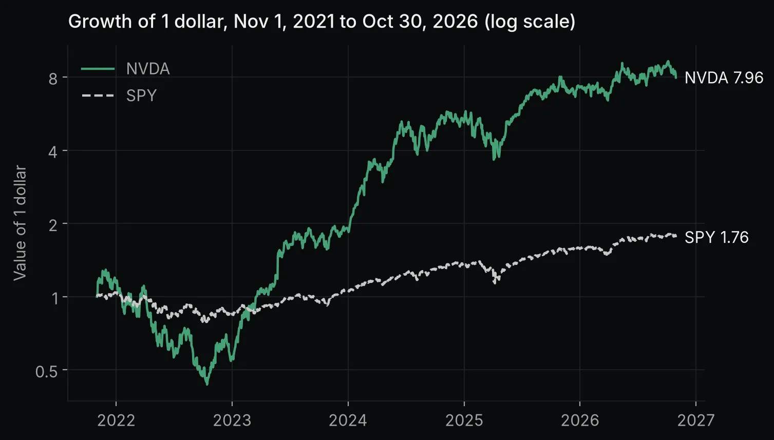 Chart made by this post’s code from Yahoo Finance data (via yfinance, unofficial) through October 30, 2026. Not investment advice.
How to calculate maximum drawdown in Python
cummax holds the highest close so far at every date. Dividing each close by it and subtracting 1 gives the drawdown, how far the price sits below its previous high. The deepest value is the maximum drawdown. The loop also finds the peak before it and the first later close at or above that peak.
drawdown = prices / prices.cummax() - 1

for t in prices:
    trough = drawdown[t].idxmin()
    peak = prices[t][:trough].idxmax()
    back = prices[t][trough:][prices[t][trough:] >= prices[t][peak]]
    recovered = back.index[0].date() if len(back) else "not yet"
    print(f"{t}: {drawdown[t].min():.1%} from {peak.date()} to {trough.date()}, back to the peak {recovered}")

fig, ax = plt.subplots()
ax.plot(drawdown.index, drawdown["NVDA"] * 100, label="NVDA")
ax.plot(drawdown.index, drawdown["SPY"] * 100, label="SPY", linestyle="--")
ax.set_title("Drawdown from the running peak (%)")
ax.set_ylabel("Below previous high (%)")
ax.legend(loc="lower left")
fig.savefig("drawdown.png")
NVDA: -66.3% from 2021-11-29 to 2022-10-14, back to the peak 2023-05-25
SPY: -24.5% from 2022-01-03 to 2022-10-12, back to the peak 2023-12-13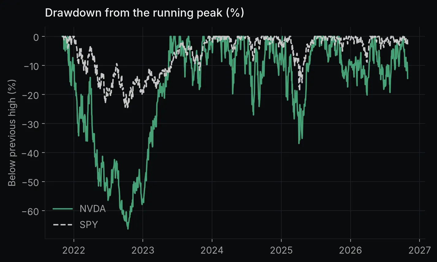 Chart made by this post’s code from Yahoo Finance data (via yfinance, unofficial) through October 30, 2026. Not investment advice.
A buyer at NVDA’s November 29, 2021 high was down 66.3% by October 14, 2022, and the stock didn’t close back at that price until May 25, 2023, the day of its 24.4% best day. SPY bottomed at -24.5% two days earlier but took until December 13, 2023 to recover. NVDA’s 695.8% five-year return includes that fall, and the total return alone doesn’t show it.
How to calculate beta and correlation in Python
Beta measures how far a stock moved for each 1% move in the market. It is the covariance of the two return series divided by the market’s variance, which is also the slope of a straight-line fit of the stock’s returns against the market’s. The code computes it both ways.
beta = returns.cov().loc["NVDA", "SPY"] / returns["SPY"].var()
slope, intercept = np.polyfit(returns["SPY"], returns["NVDA"], 1)
corr = returns.corr().loc["NVDA", "SPY"]

print(f"Beta, cov/var:     {beta:.3f}")
print(f"Beta, regression:  {slope:.3f}")
print(f"Correlation:       {corr:.3f}")
print(f"R-squared:         {corr ** 2:.3f}")
Beta, cov/var: 2.139
Beta, regression: 2.139
Correlation: 0.708
R-squared: 0.501Both methods give 2.139: over these five years NVDA moved about 2.14% for each 1% move in SPY, on average. A correlation of 0.708 squares to an R-squared of 0.501, so SPY’s moves line up with about half of the variation in NVDA’s daily returns. The other half is specific to NVDA.
Rolling one-year beta
A single beta averages five years into one number. A rolling beta recomputes it over the previous 252 trading days at every date, so the first value appears a year into the data.
rolling_beta = (returns["NVDA"].rolling(252).cov(returns["SPY"])
                / returns["SPY"].rolling(252).var()).dropna()

print(f"lowest  {rolling_beta.min():.2f} on {rolling_beta.idxmin().date()}")
print(f"highest {rolling_beta.max():.2f} on {rolling_beta.idxmax().date()}")
print(f"latest  {rolling_beta.iloc[-1]:.2f} on {rolling_beta.index[-1].date()}")

fig, ax = plt.subplots()
ax.plot(rolling_beta.index, rolling_beta)
ax.axhline(1, color="#808080", linewidth=0.8)
ax.set_title("NVDA's beta to SPY over the previous 252 trading days")
ax.set_ylabel("Beta")
fig.savefig("rolling-beta.png")
lowest 1.68 on 2026-03-30
highest 2.92 on 2025-02-19
latest 1.93 on 2026-10-30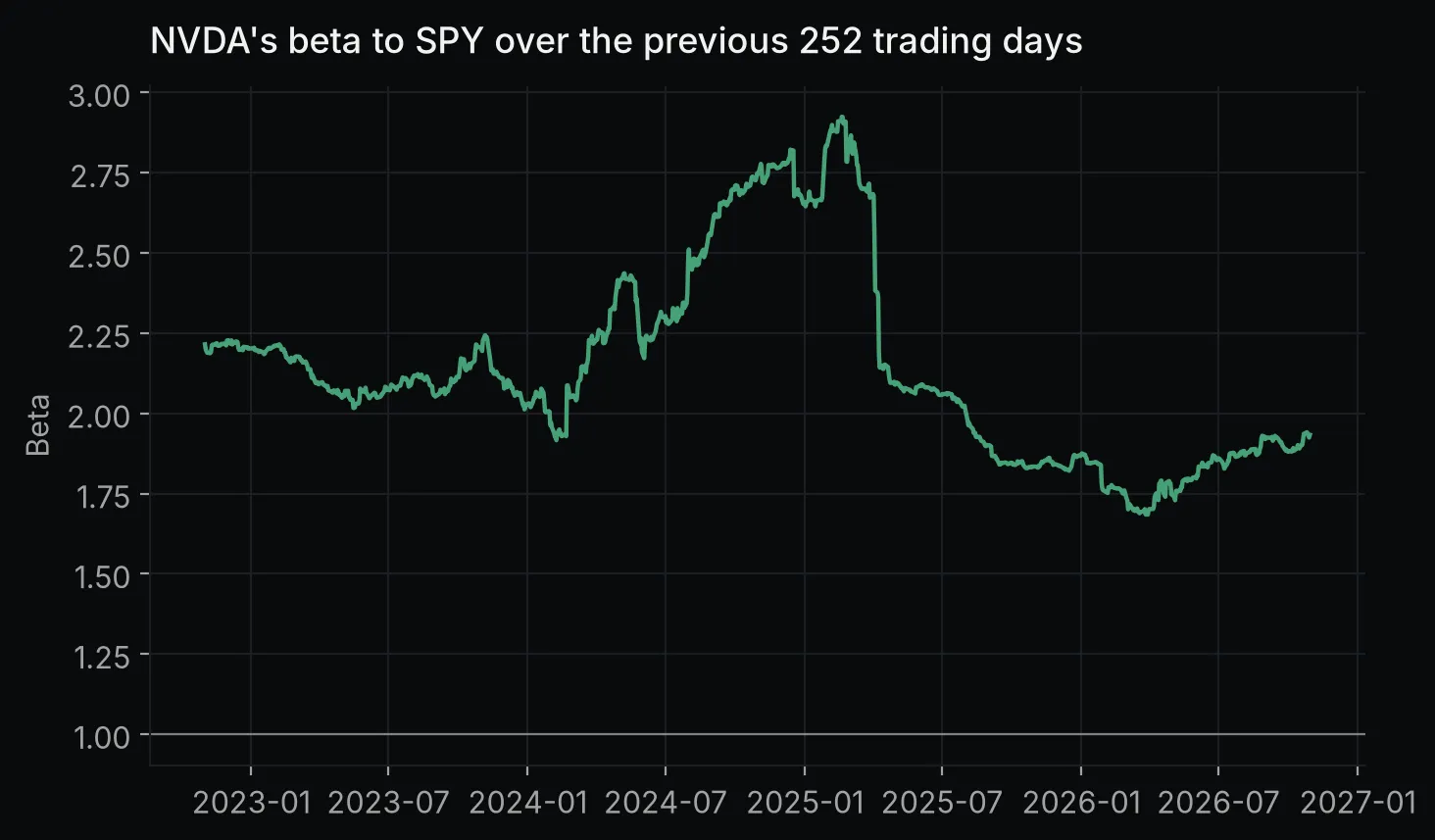 Chart made by this post’s code from Yahoo Finance data (via yfinance, unofficial) through October 30, 2026. Not investment advice.
NVDA’s one-year beta ranged from 1.68 to 2.92 and stood at 1.93 on October 30, 2026. A beta quoted for a stock depends on the window behind it.
Returns by calendar year
resample("YE") groups the closes by calendar year and .last() keeps each year’s final close; pct_change then gives each year’s return. 2021 drops out because the data starts in November. pandas 3.1.0 accepts only "YE" for year-end here: "Y" and "A", which older code uses, raise a ValueError.
yearly = prices.resample("YE").last().pct_change().dropna()
yearly.index = [str(y) if y < 2026 else "2026 to Oct 30" for y in yearly.index.year]
print(yearly.map("{:.1%}".format))
Ticker NVDA SPY
2022 -50.3% -18.2%
2023 239.0% 26.2%
2024 171.2% 24.9%
2025 38.9% 17.7%
2026 to Oct 30 10.0% 11.7%NVDA lost 50.3% in 2022 and gained 239.0% in 2023. SPY finished ahead of NVDA in 2022 and in 2026 through October 30.
FAQ
Is Python good for financial analysis?
For return and risk measures like these, yes. Each one in this post takes one to three lines of pandas, and changing the tickers or dates in yf.download reruns the whole analysis. The weak point is the data: yfinance is unofficial, and Yahoo’s terms cover what it returns.
Why does yfinance give a KeyError for Adj Close?
yf.download defaults to auto_adjust=True, which returns a Close column already adjusted for dividends and leaves out Adj Close. Use ["Close"], or pass auto_adjust=False to get both columns back.
Why does yfinance return two-level columns for one ticker?
download labels every column with a (field, ticker) pair by default, however many tickers you ask for. Select a field first, as in prices["Close"], or pass multi_level_index=False for plain column names.
Should I use simple or log returns?
This post uses simple returns from pct_change because they are what a holder earns over a day, and they add up across the stocks in a portfolio. Log returns add up across time instead, which makes them the usual choice for volatility models and simulations; quantitative finance in Python works with them.
Is yfinance free to use?
The library is free and open source under the Apache 2.0 license. Its README says it is not affiliated with Yahoo and is meant for research and educational use. It also says the Yahoo Finance API “is intended for personal use only”, and the data itself stays under Yahoo’s terms.
Where to go next
For company fundamentals instead of prices, financial modeling with Python builds a discounted cash flow model from SEC filings. The Python for finance guide maps the rest of the series, from NPV and IRR to option pricing.