
Financial Modeling With Python: Build a DCF From SEC Data
Financial modeling with Python means pulling a company’s reported numbers into pandas and turning assumptions into values with code you can rerun. This tutorial builds a discounted cash flow (DCF) model of Microsoft from SEC EDGAR’s free XBRL data, traces every input to its 10-K accession number, and shows how far the result moves with the assumptions.
Every code block on this page was run on November 4, 2026, in the order shown, and each output is pasted from that run. Versions: Python 3.13.8, pandas 3.1.0, requests 2.34.2, numpy-financial 1.1.0 and matplotlib 3.11.2. Financial data is from SEC EDGAR’s CompanyFacts API, through Microsoft’s fiscal 2026 10-K filed July 29, 2026; the SEC, Investor.gov and NYU Stern pages quoted below and the 10-K’s text were checked the same day. The growth, discount and terminal rates are illustrative assumptions, not forecasts. The model’s output is not a fair value or a price target for Microsoft, and nothing here is a recommendation to buy or sell.
Key takeaways
- SEC’s CompanyFacts API is free with no key, but it returns 403 to the default
requestsUser-Agent. Send a name and email, as SEC’s developer pages ask. - Each figure appears in several filings: Microsoft’s FY2024 operating cash flow is in three 10-Ks and an 8-K. Keep 10-K, full-year rows and one value per period end.
- Microsoft’s FY2026 operating cash flow rose to 182.9 billion dollars while capital spending reached 115.9 billion, so free cash flow fell to 67.0 billion and its margin to 20.2%.
- In the base case the terminal value is 78% of the enterprise value, so the long-run assumptions matter more than the five projected years.
- Across discount rates of 8% to 10% and terminal growth of 2% to 4%, the model’s value per share runs from 165.05 to 309.68. Counting stock pay as a cost and finance leases as debt moves the base case from 213.38 to 165.81. These are outputs of illustrative assumptions, not a fair value.
Get a company’s financial data from the SEC EDGAR API
The CompanyFacts endpoint returns every XBRL fact a company has filed, as one JSON file per company. XBRL is the tagged data format for financial statements that SEC first required in 2009, according to its EDGAR API page. Each number arrives with a name, a period and the filing it came from. The file is keyed by the company’s Central Index Key (CIK), SEC’s 10-digit ID for each filer, including leading zeros. Microsoft’s is 0000789019; SEC’s company_tickers.json maps every ticker to its CIK.
To follow along, install the libraries with pip install requests pandas numpy-financial matplotlib and run the blocks in order in one session or notebook, since each block uses variables from the ones before it.
import requests
import pandas as pd
import numpy_financial as npf
import matplotlib.pyplot as plt

url = "https://data.sec.gov/api/xbrl/companyfacts/CIK0000789019.json"
print("default User-Agent:", requests.get(url, timeout=30).status_code)

headers = {"User-Agent": "Your Name your.email@example.com"}
r = requests.get(url, headers=headers, timeout=30)
facts = r.json()
print("declared User-Agent:", r.status_code, facts["entityName"])
default User-Agent: 403
declared User-Agent: 200 MICROSOFT CORPWith the User-Agent that requests sends by default, SEC refuses the request with a 403 Forbidden. SEC’s developer FAQ asks scripts to “declare your user agent in request headers” with a company name and an admin email, and caps access at 10 requests per second. Put your own name and email in the placeholder. To pull many companies, the EDGAR API page points to a bulk companyfacts.zip, recompiled nightly, as “the most efficient means to fetch large amounts of API data.”
Why does the same number appear several times?
A 10-K is the annual report a US public company files with SEC, beside quarterly 10-Q reports and 8-K “current reports” on major events, as Investor.gov describes them. Every 10-K repeats earlier years as comparatives, so one figure shows up in several filings. Here is every row for Microsoft’s operating cash flow in the fiscal year that ended June 30, 2024:
raw = pd.DataFrame(facts["facts"]["us-gaap"]["NetCashProvidedByUsedInOperatingActivities"]["units"]["USD"])
print(raw[raw["end"] == "2024-06-30"][["start", "end", "val", "fy", "fp", "form", "filed"]].to_string(index=False))
start end val fy fp form filed
2023-07-01 2024-06-30 118548000000 2024.0 FY 10-K 2024-07-30
2023-07-01 2024-06-30 118548000000 NaN NaN 8-K 2024-12-03
2023-07-01 2024-06-30 118548000000 2025.0 FY 10-K 2025-07-30
2023-07-01 2024-06-30 118548000000 2026.0 FY 10-K 2026-07-29The same 118,548,000,000 comes from three 10-Ks and an 8-K filed on December 3, 2024. The fy column is the fiscal year of the filing, not of the number: the fiscal 2026 10-K tags this fiscal 2024 figure with fy 2026. Filtering on fy == 2024 would miss the latest copy and pick up the wrong years from other filings.
A helper that keeps one value per year
The helper keeps 10-K rows for full fiscal years, then one row per period end, taking the most recently filed value so a restated figure wins over the original. The duration filter matters because 10-Ks also tag some quarterly figures. The form filter matters too: Microsoft’s first-quarter fiscal 2027 10-Q, filed October 28, 2026, is already in the same JSON, and leaving it out keeps the model on full fiscal years.
def annual(concept, unit="USD", taxonomy="us-gaap"):
    rows = pd.DataFrame(facts["facts"][taxonomy][concept]["units"][unit])
    rows = rows[(rows["form"] == "10-K") & (rows["fp"] == "FY")]
    if "start" in rows:
        days = (pd.to_datetime(rows["end"]) - pd.to_datetime(rows["start"])).dt.days
        rows = rows[days > 360]
    rows = rows.sort_values("filed").drop_duplicates("end", keep="last")
    return rows.set_index("end").sort_index()[["val", "accn", "filed"]]

print(annual("NetCashProvidedByUsedInOperatingActivities").tail(3))
val accn filed
end
2024-06-30 118548000000 0001193125-26-323660 2026-07-29
2025-06-30 136162000000 0001193125-26-323660 2026-07-29
2026-06-30 182935000000 0001193125-26-323660 2026-07-29The accession number names the filing a value came from. All three come from 0001193125-26-323660, the fiscal 2026 10-K, which is the latest filing to report each of those years.
How do you calculate free cash flow from SEC data?
Free cash flow isn’t a line in the financial statements, so its definition is a modeling choice. Here, for each of the last ten fiscal years, it is operating cash flow minus capital spending, the PaymentsToAcquirePropertyPlantAndEquipment concept, which Microsoft’s cash flow statement calls “Additions to property and equipment”.
hist = pd.DataFrame({
    "revenue": annual("RevenueFromContractWithCustomerExcludingAssessedTax")["val"],
    "operating cash flow": annual("NetCashProvidedByUsedInOperatingActivities")["val"],
    "capex": annual("PaymentsToAcquirePropertyPlantAndEquipment")["val"],
}).loc["2017-06-30":] / 1e9
hist["free cash flow"] = hist["operating cash flow"] - hist["capex"]
hist["FCF margin"] = hist["free cash flow"] / hist["revenue"]
hist.index = [f"FY{e[:4]}" for e in hist.index]
print(hist.to_string(float_format="{:.1f}".format, formatters={"FCF margin": "{:.1%}".format}))
revenue operating cash flow capex free cash flow FCF margin
FY2017 96.6 39.5 8.1 31.4 32.5%
FY2018 110.4 43.9 11.6 32.3 29.2%
FY2019 125.8 52.2 13.9 38.3 30.4%
FY2020 143.0 60.7 15.4 45.2 31.6%
FY2021 168.1 76.7 20.6 56.1 33.4%
FY2022 198.3 89.0 23.9 65.1 32.9%
FY2023 211.9 87.6 28.1 59.5 28.1%
FY2024 245.1 118.5 44.5 74.1 30.2%
FY2025 281.7 136.2 64.6 71.6 25.4%
FY2026 331.8 182.9 115.9 67.0 20.2%Figures are in billions of dollars. From FY2017 to FY2024 the free cash flow margin stayed between 28.1% and 33.4%. In the next two years capital spending went from 44.5 billion to 115.9 billion, and the margin fell to 20.2% even as operating cash flow reached 182.9 billion. For a DCF, that makes the choice of starting year a large assumption in itself.
fig, ax = plt.subplots()
ax.plot(hist.index, hist["operating cash flow"], marker="o", label="Operating cash flow")
ax.plot(hist.index, hist["capex"], marker="o", linestyle="--", label="Capital spending")
for col in ["operating cash flow", "capex"]:
ax.annotate(f"{hist[col].iloc[-1]:.1f}", (len(hist) - 1, hist[col].iloc[-1]), xytext=(8, 0),
textcoords="offset points", va="center")
ax.set_title("Microsoft operating cash flow and capital spending, FY2017 to FY2026")
ax.set_ylabel("Billions of dollars")
ax.legend(loc="upper left")
fig.savefig("cash-flow-capex.png")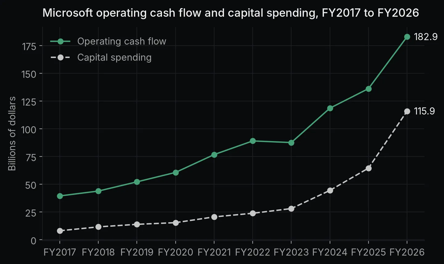 Chart made by this post’s code from SEC EDGAR data through Microsoft’s fiscal year ended June 30, 2026. Not investment advice.
Pull the model’s inputs with their sources
Each input is printed with its period and accession number, so anyone can open the filing and find it. Shares outstanding come from the 10-K’s cover page, which uses the dei taxonomy instead of us-gaap.
latest = "2026-06-30"
inputs = {
    "operating cash flow": annual("NetCashProvidedByUsedInOperatingActivities").loc[latest],
    "capex": annual("PaymentsToAcquirePropertyPlantAndEquipment").loc[latest],
    "cash and short-term investments": annual("CashCashEquivalentsAndShortTermInvestments").loc[latest],
    "debt, including current portion": annual("LongTermDebt").loc[latest],
    "finance lease liabilities": annual("FinanceLeaseLiability").loc[latest],
    "stock-based compensation": annual("ShareBasedCompensation").loc[latest],
}
shares_row = annual("EntityCommonStockSharesOutstanding", unit="shares", taxonomy="dei").iloc[-1]

for name, row in inputs.items():
    print(f"{name:33} {row['val'] / 1e9:8.3f} B  as of {latest}  accession {row['accn']}")
print(f"{'shares outstanding':33} {shares_row['val'] / 1e9:8.3f} B  as of {shares_row.name}  accession {shares_row['accn']}")
operating cash flow 182.935 B as of 2026-06-30 accession 0001193125-26-323660
capex 115.948 B as of 2026-06-30 accession 0001193125-26-323660
cash and short-term investments 76.843 B as of 2026-06-30 accession 0001193125-26-323660
debt, including current portion 40.294 B as of 2026-06-30 accession 0001193125-26-323660
finance lease liabilities 66.594 B as of 2026-06-30 accession 0001193125-26-323660
stock-based compensation 12.405 B as of 2026-06-30 accession 0001193125-26-323660
shares outstanding 7.426 B as of 2026-07-23 accession 0001193125-26-323660The 10-K’s cash flow statement shows “Net cash from operations” of 182,935 and “Additions to property and equipment” of (115,948), in millions, and its cover page counts 7,425,545,491 shares as of July 23, 2026. The base model uses the first five lines.
Two more come in for the last sensitivity check. Finance lease liabilities, at 66.594 billion, are larger than the 40.294 billion of debt. Stock-based compensation, 12.405 billion, is an expense that operating cash flow adds back because it is paid in shares, not cash.
How do you build a DCF model in Python?
A DCF projects free cash flow for a few years and discounts it at the weighted average cost of capital (WACC, the return investors require). It then adds a terminal value for everything after the last projected year. The terminal value here uses the Gordon growth formula: the year-5 cash flow times (1 + g), divided by (WACC - g). Enterprise value plus cash minus debt gives equity value, and dividing by shares gives a value per share.
The base case assumes 10% growth for five years, a 9% WACC and 3% terminal growth, all illustrative.
npf.npv treats the first value as today, so the cash flows go in after a leading 0 and year 1 is discounted one full year. NumPy financial functions covers that timing in detail.
fcf0 = (inputs["operating cash flow"]["val"] - inputs["capex"]["val"]) / 1e9
cash = inputs["cash and short-term investments"]["val"] / 1e9
debt = inputs["debt, including current portion"]["val"] / 1e9
leases = inputs["finance lease liabilities"]["val"] / 1e9
sbc = inputs["stock-based compensation"]["val"] / 1e9
shares = shares_row["val"] / 1e9

def dcf(wacc, terminal_growth, growth=0.10, start_fcf=fcf0, claims=debt, years=5):
    fcf = [start_fcf * (1 + growth) ** t for t in range(1, years + 1)]
    pv_fcf = npf.npv(wacc, [0] + fcf)
    terminal = fcf[-1] * (1 + terminal_growth) / (wacc - terminal_growth)
    pv_terminal = terminal / (1 + wacc) ** years
    ev = pv_fcf + pv_terminal
    equity = ev + cash - claims
    return {"fcf": fcf, "pv_fcf": pv_fcf, "pv_terminal": pv_terminal, "ev": ev,
            "equity": equity, "per_share": equity / shares}

base = dcf(wacc=0.09, terminal_growth=0.03)
print(f"FY2026 free cash flow:      {fcf0:.3f} B")
print(f"projected, years 1-5:       {', '.join(f'{x:.1f}' for x in base['fcf'])} B")
print(f"PV of years 1-5:            {base['pv_fcf']:.1f} B")
print(f"PV of terminal value:       {base['pv_terminal']:.1f} B ({base['pv_terminal'] / base['ev']:.0%} of the total)")
print(f"enterprise value:           {base['ev']:.1f} B")
print(f"equity value:               {base['equity']:.1f} B")
print(f"per share:                  {base['per_share']:.2f}")
FY2026 free cash flow: 66.987 B
projected, years 1-5: 73.7, 81.1, 89.2, 98.1, 107.9 B
PV of years 1-5: 344.3 B
PV of terminal value: 1203.7 B (78% of the total)
enterprise value: 1547.9 B
equity value: 1584.5 B
per share: 213.38The five projected years are worth 344.3 billion today and the terminal value 1,203.7 billion, 78% of the 1,547.9 billion enterprise value. Equity value is higher than enterprise value because Microsoft’s cash and short-term investments exceed its debt. The 213.38 per share is what these particular assumptions imply, starting from a year when capital spending rose from 64.6 billion to 115.9 billion. It is not an estimate of what the stock is worth.
How sensitive is the DCF to its assumptions?
A sensitivity table reruns the model across a grid of assumptions. Here the rows are WACC and the columns terminal growth, followed by three growth rates for the projected years and one stricter definition of free cash flow and debt.
waccs, growths = [0.08, 0.09, 0.10], [0.02, 0.03, 0.04]
grid = pd.DataFrame({f"g {g:.0%}": [dcf(w, g)["per_share"] for w in waccs] for g in growths},
                    index=[f"WACC {w:.0%}" for w in waccs])
print(grid.round(2))
print()
for growth in (0.05, 0.10, 0.15):
    label = f"FCF growth of {growth:.0%} a year:"
    print(f"{label:45} {dcf(0.09, 0.03, growth=growth)['per_share']:.2f} per share")
strict = dcf(0.09, 0.03, start_fcf=fcf0 - sbc, claims=debt + leases)
print(f"{'stock pay as a cost, finance leases as debt:':45} {strict['per_share']:.2f} per share")
g 2% g 3% g 4%
WACC 8% 220.69 256.29 309.68
WACC 9% 188.88 213.38 247.69
WACC 10% 165.05 182.77 206.39
FCF growth of 5% a year: 173.76 per share
FCF growth of 10% a year: 213.38 per share
FCF growth of 15% a year: 260.49 per share
stock pay as a cost, finance leases as debt: 165.81 per shareMoving WACC and terminal growth by one point each spans 165.05 to 309.68, almost a factor of two, and the top-right corner is where the gap between WACC and g is narrowest. Changing one assumption at a time from the 213.38 base case:
| Assumption changed | Range tested | Value per share |
|---|---|---|
| WACC, terminal growth held at 3% | 10% to 8% | 182.77 to 256.29 |
| Terminal growth, WACC held at 9% | 2% to 4% | 188.88 to 247.69 |
| Free cash flow growth in years 1 to 5 | 5% to 15% | 173.76 to 260.49 |
| Definitions of free cash flow and debt | stock pay as a cost, finance leases as debt | 165.81 |
Treating stock-based compensation as a cash cost and finance leases as debt, both defensible choices, takes the base case from 213.38 to 165.81 without touching a single rate.
A DCF is a way to see which assumptions drive a value. In this one every rate and both definitional choices move the result a long way, so a value per share means little without the assumptions printed next to it.
FAQ
Is the SEC EDGAR API free?
Yes. SEC’s EDGAR API page says the data.sec.gov APIs, CompanyFacts included, “do not require any authentication or API keys to access,” and lists the other endpoints. SEC asks for a User-Agent with a name and email and allows up to 10 requests per second.
How do I find a company’s CIK?
SEC’s company_tickers.json maps tickers to CIKs; Microsoft’s entry is 789019. The CompanyFacts URL needs it padded with zeros to 10 digits, as in CIK0000789019.
What is a good terminal growth rate for a DCF?
One the company could sustain forever, which caps it at the economy’s growth. Aswath Damodaran’s valuation notes at NYU Stern say no firm can grow forever faster than the economy it operates in. His rule of thumb is that the stable growth rate “should not exceed the riskless rate used in the valuation.” The choice carries weight: here the terminal value is 78% of enterprise value, and terminal growth of 2% or 4% at a 9% WACC gives 188.88 or 247.69 per share.
Why build a financial model in Python instead of Excel?
The data pull, the model and the sensitivity table rerun together when a new 10-K comes out, every input carries its accession number, and testing another company means changing one CIK. A spreadsheet can do the same arithmetic, but refreshing it and tracing each number back to its filing is manual work.
Where to go next
For market data instead of filings, Python for financial analysis covers returns, drawdown and beta, and the QuantLib tutorial discounts a bond with a full Treasury curve instead of a single rate. The Python for finance guide maps the rest of the series.