
QuantLib Python Tutorial: Price an Option and a Bond
QuantLib Python is the Python package for QuantLib, the open-source C++ library for pricing derivatives, bonds and yield curves: pip install QuantLib, then import QuantLib as ql. This tutorial on version 1.44 sets the evaluation date, prices a European call and checks it against Black-Scholes by hand, then prices a bond off the October 30, 2026 Treasury curve.
Every code block on this page was run on November 4, 2026 with Python 3.13.8, QuantLib 1.44, SciPy 1.18.1, pandas 3.1.0 and matplotlib 3.11.2, in the order shown. Each output is pasted from that run. Treasury yields are from FRED (Federal Reserve Bank of St. Louis) for October 30, 2026. The option’s inputs and the 4% bond are made up for the example, and nothing here is a recommendation to buy or sell anything.
Key takeaways
pip install QuantLibinstalls 1.44, released October 13, 2026, as a prebuilt wheel for Python 3.9 and newer, so there is nothing to compile.- Set
ql.Settings.instance().evaluationDatebefore anything else. Left alone, it is the day the script runs, and prices move with it. - QuantLib’s analytic engine and a hand-written Black-Scholes formula give the same call price, 5.537025, to within 2.7e-15.
vega()is per 1.00 of volatility, which is 100 percentage points. Divide by 100 for the change per point.- FRED’s Treasury yields are par yields, not zero rates. Bootstrapped into a curve, they price a 5-year bond with a 4.71% coupon at exactly 100 and a 4% bond at 96.8640.
Install QuantLib for Python
pip install QuantLib installs the package. The import name is QuantLib, usually shortened to ql.
import QuantLib as ql
print(ql.__version__)1.44Version 1.44 came out on October 13, 2026. PyPI has wheels for Windows, macOS and Linux built against Python’s stable ABI (tagged cp39-abi3), so the same file installs on Python 3.9 and every later version, 3.13 included, with no C++ compiler. QuantLib is free software under the modified BSD license. QuantLib’s home page describes it as a library “for modeling, trading, and risk management in real-life”, written in C++ and exported to C#, Java, Python and R.
Set the evaluation date first
Every QuantLib price is computed as of one global evaluation date. Unless you set it, that date is the day the script runs:
print("before:", ql.Settings.instance().evaluationDate)
today = ql.Date(30, ql.October, 2026)
ql.Settings.instance().evaluationDate = today
print("after: ", ql.Settings.instance().evaluationDate)
before: November 4th, 2026
after: October 30th, 2026The “before” line shows the run date, November 4, 2026; yours will show the day you run it. Everything below is pinned to Friday, October 30, 2026, so the prices don’t drift from one day to the next. It is the last trading day of the month and the date of the Treasury yields used later. Set the date once, at the top, before building any curve or instrument.
Calendars, business days and day counters
A calendar knows a market’s holidays. UnitedStates(ql.UnitedStates.NYSE) is the stock exchange’s; UnitedStates(ql.UnitedStates.GovernmentBond), used for the bond later, is the Treasury market’s.
nyse = ql.UnitedStates(ql.UnitedStates.NYSE)
print("Thanksgiving a business day?", nyse.isBusinessDay(ql.Date(26, ql.November, 2026)))
print("One month after today:      ", nyse.advance(today, ql.Period(1, ql.Months)))
print("One business day after:     ", nyse.advance(today, 1, ql.Days))
print("Business days to Dec 31:    ", nyse.businessDaysBetween(today, ql.Date(31, ql.December, 2026)))
print("Holidays left in 2026:      ", [str(d) for d in nyse.holidayList(today, ql.Date(31, ql.December, 2026))])

end = ql.Date(30, ql.April, 2027)
for dc in [ql.Actual365Fixed(), ql.Actual360(), ql.Thirty360(ql.Thirty360.BondBasis)]:
    print(f"{dc.name():20} {dc.dayCount(today, end)} days, {dc.yearFraction(today, end):.6f} years")
Thanksgiving a business day? False
One month after today: November 30th, 2026
One business day after: November 2nd, 2026
Business days to Dec 31: 42
Holidays left in 2026: ['November 26th, 2026', 'December 25th, 2026']
Actual/365 (Fixed) 182 days, 0.498630 years
Actual/360 182 days, 0.505556 years
30/360 (Bond Basis) 180 days, 0.500000 yearsOne business day after Friday, October 30 is Monday, November 2, and only Thanksgiving and Christmas are left as NYSE holidays in 2026. Day counters turn two dates into a fraction of a year, and the conventions disagree: the same six months is 0.498630 years on Actual/365, 0.505556 on Actual/360 and 0.500000 on 30/360. The option below uses Actual/365 Fixed. The bond uses Actual/Actual (ActualActual.Bond), which makes each semiannual coupon exactly half the annual rate.
How to price a European option in QuantLib
A QuantLib price has three parts: the instrument (what is priced), the market data (quotes and curves) and a pricing engine (how it is priced). The example is a six-month call struck at 105 on a stock at 100, with 25% volatility, a 4% risk-free rate and a 1% dividend yield, all made up.
expiry = ql.Date(30, ql.April, 2027)
spot, strike, vol, rate, div = 100.0, 105.0, 0.25, 0.04, 0.01
dc = ql.Actual365Fixed()

spot_quote = ql.SimpleQuote(spot)
process = ql.BlackScholesMertonProcess(
    ql.QuoteHandle(spot_quote),
    ql.YieldTermStructureHandle(ql.FlatForward(today, div, dc)),
    ql.YieldTermStructureHandle(ql.FlatForward(today, rate, dc)),
    ql.BlackVolTermStructureHandle(ql.BlackConstantVol(today, nyse, vol, dc)),
)
option = ql.VanillaOption(ql.PlainVanillaPayoff(ql.Option.Call, strike), ql.EuropeanExercise(expiry))
option.setPricingEngine(ql.AnalyticEuropeanEngine(process))

print(f"price  {option.NPV():.6f}")
print(f"delta  {option.delta():.6f}")
print(f"gamma  {option.gamma():.6f}")
print(f"vega   {option.vega():.6f} per 1.00 of volatility, {option.vega() / 100:.6f} per point")
print(f"theta  {option.thetaPerDay():.6f} per day")
price 5.537025
delta 0.456551
gamma 0.022366
vega 27.881320 per 1.00 of volatility, 0.278813 per point
theta -0.022295 per dayBlackScholesMertonProcess bundles the spot, a dividend-yield curve, an interest-rate curve (both flat and continuously compounded here) and the volatility. AnalyticEuropeanEngine is the closed-form Black-Scholes-Merton formula. The call is worth 5.537025 with a delta of 0.456551.
The Greeks measure how the price responds to its inputs. Delta, 0.456551, is roughly what the call gains for a 1.00 rise in the stock, and gamma, 0.022366, is how fast delta itself changes. Mind the units on the other two. vega() is the price change for a change of 1.00 in volatility, from 25% to 125%, so a one-point rise in volatility adds about 0.278813. thetaPerDay() is the value lost as one day passes; theta() without the suffix is the same figure per year.
Check it against Black-Scholes by hand
The same price from the formula, with SciPy’s normal distribution:
from math import exp, log, sqrt
from scipy.stats import norm

T = dc.yearFraction(today, expiry)
d1 = (log(spot / strike) + (rate - div + vol ** 2 / 2) * T) / (vol * sqrt(T))
d2 = d1 - vol * sqrt(T)
call = spot * exp(-div * T) * norm.cdf(d1) - strike * exp(-rate * T) * norm.cdf(d2)
delta = exp(-div * T) * norm.cdf(d1)

print(f"T      {T:.6f} years")
print(f"price  {call:.6f}")
print(f"delta  {delta:.6f}")
print(f"difference from QuantLib: {abs(call - option.NPV()):.1e}")
T 0.498630 years
price 5.537025
delta 0.456551
difference from QuantLib: 2.7e-15The two agree to 2.7e-15, which is floating-point rounding. T comes from the same day counter, so both sides use 182 days out of 365.
Implied volatility and live quotes
impliedVolatility runs the model backwards: it finds the volatility at which the call would be worth a given price. And because the spot went in as a SimpleQuote, changing the quote reprices the option without rebuilding anything.
print(f"implied vol at a price of 6.00: {option.impliedVolatility(6.00, process):.4%}")

spot_quote.setValue(110.0)
print(f"price with the stock at 110:    {option.NPV():.6f}")
spot_quote.setValue(100.0)
print(f"back at 100:                    {option.NPV():.6f}")
implied vol at a price of 6.00: 26.6578%
price with the stock at 110: 11.179168
back at 100: 5.537025A price of 6.00 implies 26.6578% volatility. With the stock at 110 the call is worth 11.179168, and setting the quote back restores 5.537025. This is how QuantLib handles live data: instruments watch their quotes and recalculate when one changes.
Get Treasury yields from FRED
FRED publishes the Treasury’s daily constant-maturity yields, from the Federal Reserve’s H.15 release, as series DGS1MO through DGS30. Asking fredgraph.csv for several series at once returns their full history in one CSV, with no API key, and pandas picks out the day.
import pandas as pd

tenors = {"DGS1MO": ql.Period(1, ql.Months), "DGS3MO": ql.Period(3, ql.Months),
          "DGS6MO": ql.Period(6, ql.Months), "DGS1": ql.Period(1, ql.Years),
          "DGS2": ql.Period(2, ql.Years), "DGS3": ql.Period(3, ql.Years),
          "DGS5": ql.Period(5, ql.Years), "DGS7": ql.Period(7, ql.Years),
          "DGS10": ql.Period(10, ql.Years), "DGS20": ql.Period(20, ql.Years),
          "DGS30": ql.Period(30, ql.Years)}
url = "https://fred.stlouisfed.org/graph/fredgraph.csv?id=" + ",".join(tenors)
fred = pd.read_csv(url, index_col="observation_date", parse_dates=True)
yields = fred.loc["2026-10-30"] / 100
print(yields.map("{:.2%}".format).to_dict())
{'DGS1MO': '4.06%', 'DGS3MO': '4.16%', 'DGS6MO': '4.25%', 'DGS1': '4.36%', 'DGS2': '4.56%', 'DGS3': '4.65%', 'DGS5': '4.71%', 'DGS7': '4.80%', 'DGS10': '4.94%', 'DGS20': '5.34%', 'DGS30': '5.31%'}These are par yields. The Treasury’s yield curve methodology says its official curve “is a par yield curve derived using a monotone convex method”, with bill inputs on a bond-equivalent basis. A par yield is the coupon at which a bond would trade at exactly 100. Pricing a bond with any other coupon needs a zero curve: one rate for each single future payment.
Bootstrap a zero curve from par yields
Bootstrapping solves for discount factors one maturity at a time, so that each input prices exactly. The 1-month to 6-month yields go in as deposits paying simple interest on a 365-day year. The 1-year to 30-year yields go in as bonds paying that coupon twice a year and priced at 100.
Every helper pays on exact semiannual dates because the par curve describes theoretical bonds; a real Treasury whose payment date lands on a weekend pays on the next business day. PiecewiseConvexMonotoneForward interpolates between the points with a monotone convex method, the same family Treasury uses.
gov = ql.UnitedStates(ql.UnitedStates.GovernmentBond)
actact = ql.ActualActual(ql.ActualActual.Bond)

def schedule(years):
    return ql.Schedule(today, today + ql.Period(years, ql.Years), ql.Period(ql.Semiannual), gov,
                       ql.Unadjusted, ql.Unadjusted, ql.DateGeneration.Backward, False)

helpers = []
for series, tenor in tenors.items():
    y = float(yields[series])
    if tenor.units() == ql.Months:
        helpers.append(ql.DepositRateHelper(ql.QuoteHandle(ql.SimpleQuote(y)), tenor, 0, gov,
                                            ql.Unadjusted, False, ql.Actual365Fixed()))
    else:
        helpers.append(ql.FixedRateBondHelper(ql.QuoteHandle(ql.SimpleQuote(100.0)), 0, 100.0,
                                              schedule(tenor.length()), [y], actact, ql.Unadjusted))

curve = ql.PiecewiseConvexMonotoneForward(today, helpers, ql.Actual365Fixed())
curve_handle = ql.YieldTermStructureHandle(curve)

print("tenor   par    zero   discount")
for series, tenor in tenors.items():
    d = today + tenor
    zero = curve.zeroRate(d, ql.Actual365Fixed(), ql.Compounded, ql.Semiannual).rate()
    print(f"{str(tenor):6} {yields[series]:.2%}  {zero:.2%}  {curve.discount(d):.4f}")
tenor par zero discount
1M 4.06% 4.09% 0.9966
3M 4.16% 4.18% 0.9896
6M 4.25% 4.25% 0.9792
1Y 4.36% 4.36% 0.9578
2Y 4.56% 4.56% 0.9137
3Y 4.65% 4.65% 0.8710
5Y 4.71% 4.72% 0.7920
7Y 4.80% 4.82% 0.7165
10Y 4.94% 4.98% 0.6113
20Y 5.34% 5.51% 0.3372
30Y 5.31% 5.38% 0.2031Out to 7 years the zero rates sit within a few hundredths of a point of the par yields. Further out they pull away: 5.51% against 5.34% at 20 years. A 20-year par bond’s coupons are discounted at the lower rates of the earlier years, so the rate on its final payment has to be higher to bring the price to 100. The discount column is what 1 dollar paid at that maturity is worth today, 0.6113 at 10 years.
import matplotlib.pyplot as plt
t = [m / 12 for m in range(1, 361)]
zero_curve = [curve.zeroRate(x, ql.Compounded, ql.Semiannual).rate() * 100 for x in t]
par_t = [curve.timeFromReference(today + tenor) for tenor in tenors.values()]
fig, ax = plt.subplots()
ax.plot(t, zero_curve, label="Zero rate, bootstrapped")
ax.plot(par_t, yields * 100, "o", markersize=6, label="Par yield, FRED")
ax.annotate(f"zero {zero_curve[239]:.2f}%", (t[239], zero_curve[239]), xytext=(0, 10),
textcoords="offset points", ha="center")
ax.annotate(f"par {yields['DGS20']:.2%}", (par_t[9], yields["DGS20"] * 100), xytext=(0, -18),
textcoords="offset points", ha="center")
ax.set_title("US Treasury curve, October 30, 2026")
ax.set_xlabel("Years to maturity")
ax.set_ylabel("Yield, semiannual compounding (%)")
ax.legend(loc="lower right")
fig.savefig("treasury-curve.png")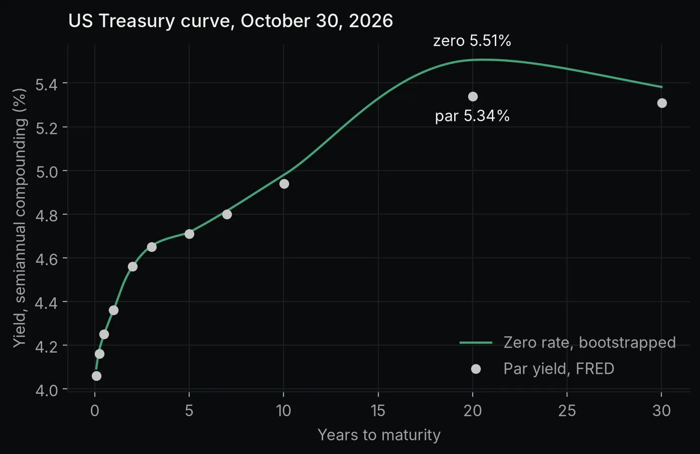 Chart made by this post’s code from FRED Treasury yield data through October 30, 2026. Not investment advice.
How to price a bond off the curve in QuantLib
First, a check that the curve does what it was built to do: a bond whose coupon equals the 5-year par yield should price at 100.
def treasury_bond(coupon, years):
    bond = ql.FixedRateBond(0, 100.0, schedule(years), [coupon], actact, ql.Unadjusted)
    bond.setPricingEngine(ql.DiscountingBondEngine(curve_handle))
    return bond

par_bond = treasury_bond(float(yields["DGS5"]), 5)
print(f"5-year bond with a {yields['DGS5']:.2%} coupon: clean price {par_bond.cleanPrice():.6f}")
5-year bond with a 4.71% coupon: clean price 100.000000Then a 5-year bond with a 4% coupon, made up for the example, on the same semiannual dates:
bond = treasury_bond(0.04, 5)
flows = bond.cashflows()
print(len(flows), "cash flows")
for cf in list(flows[:2]) + list(flows[-2:]):
    print(f"  {cf.date()}  {cf.amount():.2f}")

ytm = bond.bondYield(actact, ql.Compounded, ql.Semiannual)
ytm_rate = ql.InterestRate(ytm, actact, ql.Compounded, ql.Semiannual)
mod_dur = ql.BondFunctions.duration(bond, ytm_rate, ql.Duration.Modified)
convexity = ql.BondFunctions.convexity(bond, ytm_rate)

print(f"clean price        {bond.cleanPrice():.4f}")
print(f"yield to maturity  {ytm:.4%}")
print(f"modified duration  {mod_dur:.4f}")
print(f"convexity          {convexity:.4f}")
11 cash flows
April 30th, 2027 2.00
October 30th, 2027 2.00
October 30th, 2031 2.00
October 30th, 2031 100.00
clean price 96.8640
yield to maturity 4.7113%
modified duration 4.4676
convexity 23.2820The 11 cash flows are ten coupons of 2.00 and the 100 of principal, listed separately on the last date. The coupon is below the 4.71% par yield, so the bond prices below 100, at 96.8640, for a yield to maturity of 4.7113%. The clean price leaves out accrued interest, the coupon earned since the last payment date, and the dirty price includes it. The two are the same here because the bond is priced on the day its first coupon period starts, so nothing has accrued yet.
How much does the price move if yields rise?
Modified duration estimates the percentage price change for a change in yield, and convexity corrects for the curve in that relationship. Repricing at a yield 1 point higher shows how close each estimate gets:
price = bond.cleanPrice()
up = ql.BondFunctions.cleanPrice(bond, ytm + 0.01, actact, ql.Compounded, ql.Semiannual)
print(f"exact, yield 1 point higher:  {up:.4f}  ({up / price - 1:.3%})")
print(f"duration estimate:            {-mod_dur * 0.01:.3%}")
print(f"duration plus convexity:      {-mod_dur * 0.01 + 0.5 * convexity * 0.01 ** 2:.3%}")
exact, yield 1 point higher: 92.6471 (-4.353%)
duration estimate: -4.468%
duration plus convexity: -4.351%The exact price falls to 92.6471, a 4.353% drop. Duration alone says 4.468%, and adding the convexity term gives 4.351%, almost the exact answer.
FAQ
How do I install QuantLib in Python?
Run pip install QuantLib. Version 1.44 ships prebuilt wheels for Windows, macOS and Linux that work on Python 3.9 and newer, so no compiler or C++ build is needed. Import it with import QuantLib as ql.
Why do my QuantLib results change from day to day?
The evaluation date defaults to the day the code runs. Set ql.Settings.instance().evaluationDate to a fixed ql.Date at the top of the script, before building curves or instruments.
Can QuantLib price American options?
Yes. Replace ql.EuropeanExercise(expiry) with ql.AmericanExercise(today, expiry) and the analytic engine with a numerical one, such as ql.FdBlackScholesVanillaEngine(process) (finite differences) or ql.BinomialVanillaEngine(process, "crr", 500) (a 500-step binomial tree). Early exercise has no closed-form price in general, so AnalyticEuropeanEngine doesn’t apply.
Is QuantLib still maintained?
Yes. Version 1.44 came out on October 13, 2026, three months after 1.43 on July 14, which followed 1.42 on April 14. The QuantLib releases page on GitHub lists each one, and the Python package on PyPI is updated the same day.
Is QuantLib free for commercial use?
QuantLib is released under the modified (3-clause) BSD license, which allows use in commercial software as long as the copyright notice and license text are kept.
Where to go next
Quantitative finance in Python simulates price paths with Monte Carlo and measures risk with VaR. Financial modeling with Python discounts a company’s cash flows instead of a bond’s, and NumPy financial functions covers NPV and IRR at a single flat rate. The Python for finance guide maps the rest of the series.