
Quantitative Finance in Python: Risk Math With Code
Quantitative finance in Python starts with NumPy, pandas and SciPy applied to returns: log returns, annualized volatility, a Sharpe ratio, value at risk and Monte Carlo simulation. This tutorial computes each one on five years of SPY, tests the normal-distribution assumption several of them rely on, and simulates a hypothetical year with geometric Brownian motion.
Every code block on this page was run on November 4, 2026, in the order shown, and each output is pasted from that run. Versions: Python 3.13.8, pandas 3.1.0, NumPy 2.5.4, SciPy 1.18.1, yfinance 1.8.0 and matplotlib 3.11.2. Prices are daily closes adjusted for dividends for SPY, the State Street SPDR S&P 500 ETF Trust, a fund that tracks the S&P 500. They come from Yahoo Finance via yfinance (unofficial), November 1, 2021 to October 30, 2026, and Yahoo’s data is covered by its terms of service. The risk-free rate is the 3-month Treasury yield from FRED. Every statistic is measured in-sample on this one window, simulated results are hypothetical and not a forecast, and past returns don’t predict future ones.
Key takeaways
- Log returns add up over time: SPY’s 1,254 daily log returns sum to 0.5632, the log of its total growth. Simple returns don’t.
- SPY’s annual volatility was 17.14%, but over rolling 63-day windows it ran from 8.5% to 33.7%.
- Daily returns have fat tails: an excess kurtosis of 7.947, and 13 days beyond three standard deviations where a normal distribution expects 3.4.
- A normal 99% one-day VaR of 2.47% was beaten on 22 days against 12.5 expected. The historical 99% VaR was 2.93%.
- The Sharpe ratio was 0.51 after subtracting the 3-month Treasury yield, which averaged 3.99%. Leaving the risk-free rate out gives 0.74.
- A hypothetical 10,000-path simulation puts the median value of 1 dollar after a year at 1.1206, against 1.1198 from the closed-form formula.
Why use log returns instead of simple returns?
A simple return is today’s close over yesterday’s, minus 1. A log return is the natural log of that same ratio. They are close for small moves, but only log returns add up across time.
To follow along, install the libraries with pip install yfinance pandas numpy scipy matplotlib and run the blocks in order in one session or notebook, since each block uses variables from the ones before it.
import yfinance as yf
import pandas as pd
import numpy as np
from scipy import stats
import matplotlib.pyplot as plt

spy = yf.download("SPY", start="2021-11-01", end="2026-10-31", progress=False)["Close"]["SPY"]
simple = spy.pct_change().dropna()
log_r = np.log(spy).diff().dropna()

print(f"{len(log_r)} daily returns, {spy.index[0].date()} to {spy.index[-1].date()}")
print(f"sum of log returns:     {log_r.sum():.4f}")
print(f"log of total growth:    {np.log(spy.iloc[-1] / spy.iloc[0]):.4f}")
print(f"sum of simple returns:  {simple.sum():.4f}")
print(f"total simple return:    {spy.iloc[-1] / spy.iloc[0] - 1:.4f}")
1254 daily returns, 2021-11-01 to 2026-10-30
sum of log returns: 0.5632
log of total growth: 0.5632
sum of simple returns: 0.6365
total simple return: 0.7564The 1,254 log returns sum to 0.5632, exactly the log of SPY’s growth over the window. The simple returns sum to 0.6365, which matches nothing: the real total return was 0.7564, or 75.6%. That additivity is why log returns are the default for anything that scales or simulates returns over time, including the volatility and Monte Carlo sections below. Simple returns are still what a holder earns, and the right ones to average across stocks in a portfolio; Python for financial analysis uses them for total return, drawdown and beta.
How do you annualize volatility in Python?
To annualize volatility, multiply the standard deviation of daily returns by the square root of 252, the usual number of trading days in a year. Volatility is that standard deviation: how widely returns spread around their average. The square-root scaling assumes each day is independent of the last and equally volatile.
daily_vol = log_r.std()
print(f"daily volatility:   {daily_vol:.4%}")
print(f"annual volatility:  {daily_vol * np.sqrt(252):.2%}")

rolling = log_r.rolling(63).std() * np.sqrt(252)
print(f"63-day volatility, lowest:  {rolling.min():.1%} on {rolling.idxmin().date()}")
print(f"63-day volatility, highest: {rolling.max():.1%} on {rolling.idxmax().date()}")
daily volatility: 1.0798%
annual volatility: 17.14%
63-day volatility, lowest: 8.5% on 2025-10-03
63-day volatility, highest: 33.7% on 2025-05-28SPY’s five-year annual volatility was 17.14%. Measured over 63 trading days at a time, about three months, it ranged from 8.5% to 33.7%, and the high came in the window that takes in April 2025. Volatility comes in calm and turbulent stretches, and a single five-year number averages them away.
Are daily returns normally distributed?
Not for SPY: its daily returns have far more extreme days than a bell curve allows, and that matters because the normal VaR and the simulation below both assume one.
Two numbers measure the gap. Skewness measures lopsidedness, negative when the big moves are mostly down. Excess kurtosis measures how heavy the tails are. Both are 0 for a normal distribution.
z = (log_r - log_r.mean()) / log_r.std()
print(f"skewness:         {stats.skew(log_r):.3f}")
print(f"  without the best day ({log_r.idxmax().date()}, {log_r.max():.2%}): {stats.skew(log_r.drop(log_r.idxmax())):.3f}")
print(f"excess kurtosis:  {stats.kurtosis(log_r):.3f}")
print(f"days beyond 3 standard deviations: {(z.abs() > 3).sum()}")
print(f"a normal distribution expects:     {len(z) * 2 * stats.norm.sf(3):.1f}")

fig, ax = plt.subplots()
ax.hist(log_r * 100, bins=80, density=True, label="SPY daily log returns")
x = np.linspace(log_r.min(), log_r.max(), 400)
ax.plot(x * 100, stats.norm.pdf(x, log_r.mean(), log_r.std()) / 100, linestyle="--",
        label="Normal, same mean and SD")
ax.set_yscale("log")
ax.set_ylim(2e-3, None)
ax.set_title("SPY daily log returns vs a normal curve, Nov 2021 to Oct 2026")
ax.set_xlabel("Daily log return (%)")
ax.set_ylabel("Density (log scale)")
ax.legend(loc="upper left")
fig.savefig("return-histogram.png")
skewness: 0.162
without the best day (2025-04-09, 9.99%): -0.489
excess kurtosis: 7.947
days beyond 3 standard deviations: 13
a normal distribution expects: 3.4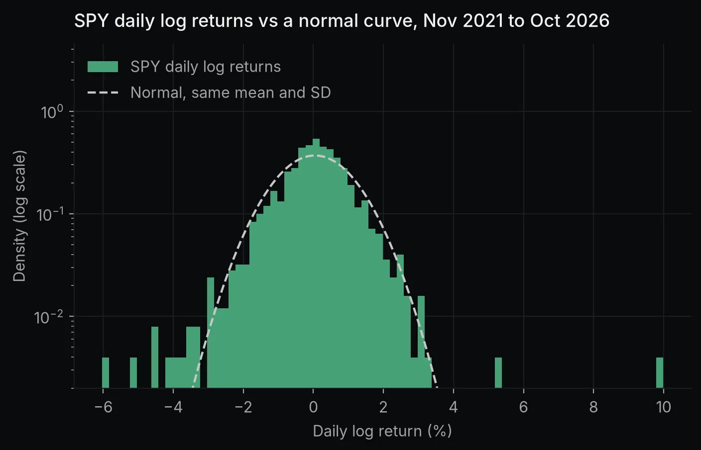 Chart made by this post’s code from Yahoo Finance data (via yfinance, unofficial) through October 30, 2026. Not investment advice.
An excess kurtosis of 7.947 means fat tails: 13 days moved more than three standard deviations, where a normal curve with the same mean and spread expects 3.4. The log scale makes it visible. The bars sit above the dashed curve near zero and again in both tails, with whole days out where the curve is almost zero. The slight positive skew, 0.162, comes from one day: without the 9.99% log return on April 9, 2025 it turns negative, -0.489, with the larger moves on the downside.
How do you calculate a Sharpe ratio in Python?
The Sharpe ratio is the average return above the risk-free rate divided by its standard deviation, annualized with the square root of 252. William Sharpe’s 1994 article on the ratio derives that square-root scaling by assuming returns with zero serial correlation, much like the assumption behind annualized volatility. The risk-free rate here is the 3-month constant-maturity Treasury yield from the Federal Reserve’s H.15 release, published on FRED as series DGS3MO and divided by 252 to approximate a daily rate.
rf_yield = pd.read_csv(
    "https://fred.stlouisfed.org/graph/fredgraph.csv?id=DGS3MO&cosd=2021-11-01&coed=2026-10-30",
    index_col="observation_date", parse_dates=True)["DGS3MO"]
rf_daily = (rf_yield / 100 / 252).reindex(simple.index).ffill()
excess = simple - rf_daily

print(f"FRED blanks in the window:        {rf_yield.isna().sum()}")
print(f"stock trading days with a blank:  {rf_yield.reindex(simple.index).isna().sum()}")
print(f"average 3-month Treasury yield:   {rf_yield.mean():.2f}%")
print(f"Sharpe ratio:                     {excess.mean() / excess.std() * np.sqrt(252):.2f}")
print(f"same ratio without the risk-free: {simple.mean() / simple.std() * np.sqrt(252):.2f}")
FRED blanks in the window: 56
stock trading days with a blank: 9
average 3-month Treasury yield: 3.99%
Sharpe ratio: 0.51
same ratio without the risk-free: 0.74FRED leaves bond-market holidays blank, 56 in this window. Nine of them were days the stock market was open, Columbus Day and Veterans Day, so the code reindexes to SPY’s trading days and carries the last yield forward. With 3-month Treasuries averaging 3.99%, subtracting the risk-free rate matters: the Sharpe ratio is 0.51 with it and 0.74 without it.
Value at risk in Python: historical vs parametric
A one-day 95% value at risk (VaR) is the loss exceeded on 5% of days. The historical version reads it straight off the past returns with a percentile. The parametric version, also called normal or variance-covariance VaR, takes the mean plus a z-score times the standard deviation. The z-score is the number of standard deviations below the mean that leaves 5% of a normal distribution beyond it. Expected shortfall, also called conditional VaR (CVaR), is the average loss on the days worse than the VaR.
for conf in (0.95, 0.99):
    hist_var = -np.percentile(simple, (1 - conf) * 100)
    normal_var = -(simple.mean() + stats.norm.ppf(1 - conf) * simple.std())
    shortfall = -simple[simple <= -hist_var].mean()
    breaches = (simple < -normal_var).sum()
    print(f"{conf:.0%} one-day VaR: historical {hist_var:.2%}, normal {normal_var:.2%}, "
          f"expected shortfall {shortfall:.2%}")
    print(f"    days worse than the normal VaR: {breaches}, expected {len(simple) * (1 - conf):.1f}")
95% one-day VaR: historical 1.66%, normal 1.73%, expected shortfall 2.46%
days worse than the normal VaR: 55, expected 62.7
99% one-day VaR: historical 2.93%, normal 2.47%, expected shortfall 3.88%
days worse than the normal VaR: 22, expected 12.5At 95% the normal VaR, 1.73%, is a little cautious: it was beaten on 55 days against 62.7 expected. At 99% it is too small, 2.47% against 2.93% from history, and was beaten on 22 days instead of 12.5. That is the fat tails from the previous section showing up in a risk number.
VaR is also a threshold, not a worst case: on the 1% of days past the historical 99% VaR, the average loss was 3.88%. Bank regulation uses that average as well: in the Basel Committee’s market-risk standard, banks using their own models compute expected shortfall at a 97.5% one-tailed confidence level (MAR33.3).
One caveat applies to all of these: they are in-sample. The historical VaR is fitted to the same days it is checked against. A fair test, called backtesting the VaR, computes it on a rolling window and counts breaches on the days that follow.
Monte Carlo simulation of a stock in Python
Geometric Brownian motion, the model behind Black-Scholes, says the log price takes independent normal steps with a constant mean and standard deviation. The simulation draws those steps from SPY’s own daily mean and spread: 10,000 paths of 252 trading days, starting from 1 dollar, with a fixed seed so the output repeats.
rng = np.random.default_rng(42)
mu, sigma = log_r.mean(), log_r.std()
days, paths = 252, 10_000

steps = rng.normal(mu, sigma, size=(days, paths))
sims = np.vstack([np.ones(paths), np.exp(np.cumsum(steps, axis=0))])
end = sims[-1]

print(f"median value of 1 dollar after a year: {np.median(end):.4f} (formula {np.exp(mu * days):.4f})")
print(f"chance of ending below 1:              {(end < 1).mean():.2%} (formula "
      f"{stats.norm.cdf(-mu * days / (sigma * np.sqrt(days))):.2%})")
print(f"5th and 95th percentile:               {np.percentile(end, 5):.4f} and {np.percentile(end, 95):.4f}")

boot = np.exp(rng.choice(log_r.to_numpy(), size=(days, paths)).sum(axis=0))
print(f"same percentiles, resampling history:  {np.percentile(boot, 5):.4f} and {np.percentile(boot, 95):.4f}")
median value of 1 dollar after a year: 1.1206 (formula 1.1198)
chance of ending below 1: 25.01% (formula 25.45%)
5th and 95th percentile: 0.8430 and 1.4878
same percentiles, resampling history: 0.8459 and 1.4860Under this model a year’s log return is normal, so the median and the chance of a loss have exact formulas, and the simulation lands close to both: 1.1206 against 1.1198, and 25.01% against 25.45%. Those checks are worth writing for any simulation, because a sign error or a wrong axis in cumsum would show up as a mismatch.
The bootstrap line, the last one in the block, resamples actual SPY days with replacement instead of drawing normal ones. Its 5th and 95th percentiles, 0.8459 and 1.4860, are almost the same, because over 252 independent draws the fat tails mostly average out. Neither version captures the stretches of high and low volatility measured above, since both draw each day independently.
q = np.percentile(sims, [5, 25, 50, 75, 95], axis=1)
d = np.arange(days + 1)
fig, ax = plt.subplots()
ax.fill_between(d, q[0], q[4], color="#45a176", alpha=0.18, linewidth=0, label="5th to 95th percentile")
ax.fill_between(d, q[1], q[3], color="#45a176", alpha=0.38, linewidth=0, label="25th to 75th percentile")
ax.plot(d, q[2], color="#45a176", label="Median")
for p, label in zip([q[0][-1], q[2][-1], q[4][-1]], ["5th", "median", "95th"]):
ax.annotate(f"{label} {p:.2f}", (days, p), xytext=(6, 0), textcoords="offset points", va="center")
ax.set_title("10,000 simulated years of 1 dollar in SPY (hypothetical)")
ax.set_xlabel("Trading days ahead")
ax.set_ylabel("Value of 1 dollar")
ax.legend(loc="upper left")
fig.savefig("monte-carlo-fan.png")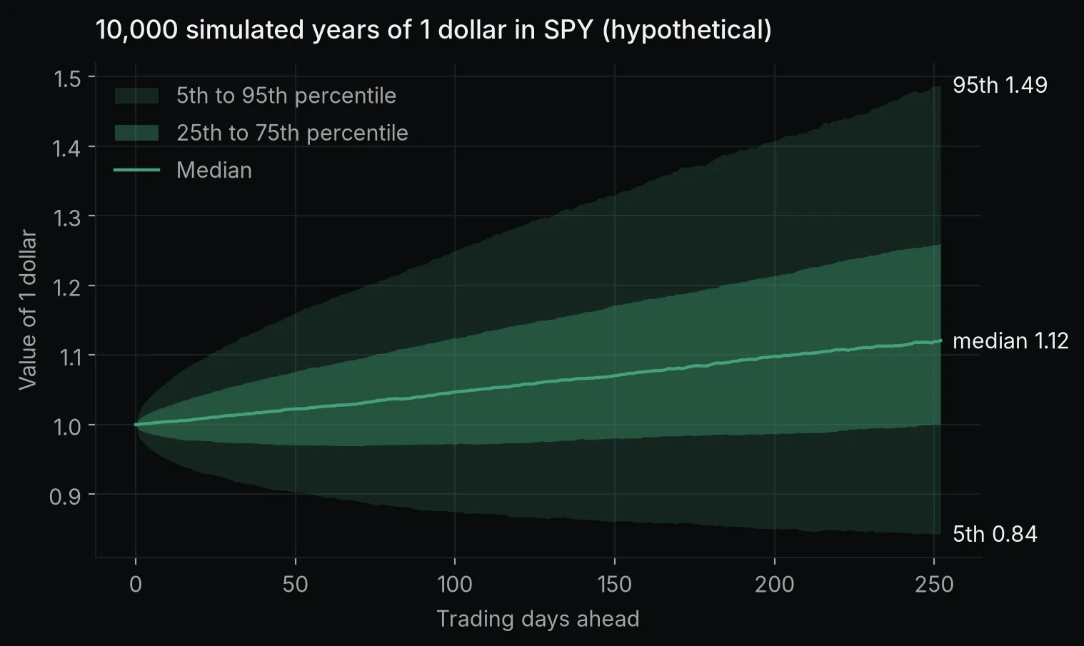 Chart made by this post’s code from Yahoo Finance data (via yfinance, unofficial) through October 30, 2026. Hypothetical simulation, not a forecast. Not investment advice.
The fan shows the model’s spread, not a prediction for SPY. It assumes the next year’s returns come from the last five years’ average and volatility, and that assumption is the part to question.
FAQ
Should I annualize volatility with 252 or 365?
Use the number of periods the asset trades in a year. US stocks and ETFs trade about 252 days a year, so daily volatility times the square root of 252 is the convention. Crypto trades every day, so analysts use 365 there.
Is value at risk the most I can lose?
No. VaR is the loss exceeded on a given share of days, so the worst days are by definition past it. Expected shortfall (CVaR), the average loss beyond the VaR, describes those days; for SPY it was 3.88% at 99%, against a VaR of 2.93%.
What is a good Sharpe ratio?
There is no fixed cutoff, because the ratio changes with the period, the return frequency and the risk-free rate. Sharpe’s 1994 article says it “is not independent of the time period over which it is measured.” Compare ratios computed the same way over the same window. Over November 2021 to October 2026, with the 3-month Treasury yield as the risk-free rate, SPY’s was 0.51.
Which Python libraries do quants use?
NumPy and pandas for the data, SciPy for distributions and optimization, and matplotlib for charts, as in this post. For pricing options, bonds and yield curves, QuantLib’s Python package adds day counters, calendars and pricing engines.
Where to go next
The Python for finance guide maps the rest of this series, from cash-flow math to building a model from SEC filings. For a structured course or a textbook to go deeper into the statistics, the list of Python for finance courses and books compares eight on prerequisites, length and price.