
Python for Finance: A Practical Guide With Real Code
Python for finance means using Python’s free data libraries, mainly pandas and NumPy, plus finance packages such as numpy-financial and QuantLib. With them you download prices and filings, measure returns and risk, price options and value companies, in code you can rerun. This guide gives the order to learn it in, with one runnable example per step.
Every code block on this page was run on November 4, 2026, in the order shown, and each output is pasted from that run. The chart in step 1 was drawn on November 17, 2026, by rerunning step 1 on the same dates, which gave the same output. The run used Python 3.13.8, pandas 3.1.0, NumPy 2.5.4, yfinance 1.8.0, numpy-financial 1.1.0, QuantLib 1.44 and requests 2.34.2, plus matplotlib 3.11.2 for the chart. Prices are daily closes from Yahoo Finance via yfinance (unofficial), covered by Yahoo’s terms of service. Company figures are from SEC EDGAR. Nothing here is investment advice, and past returns don’t predict future ones.
Key takeaways
- Learn in the order the work uses it: pandas and NumPy for data first, then risk, the time value of money, pricing and valuation.
- SPY returned 75.6% from November 1, 2021 to October 30, 2026, 11.9% a year, with 17.2% annual volatility and a worst drawdown of -24.5%. Its 95% one-day VaR was 1.66%: it lost more than that on 63 of 1,254 days.
- numpy-financial’s
npvcounts the first cash flow as today and Excel’s NPV doesn’t: 517,892.29 against 479,529.89 for the same cash flows. - SEC’s free CompanyFacts API has every figure a company reports, but each one appears in several filings: keep the 10-K rows that cover a full year, then take the latest. For Microsoft’s fiscal 2026 that gives 66,987 million dollars of free cash flow.
What should you learn first in Python for finance?
Learn the tools in the order the work uses them: load data, measure it, then price and value things with it. Each step below has one short example on this page and a full tutorial in this series.
| Step | What you learn | Libraries |
|---|---|---|
| 1. Market data | Returns, CAGR, volatility, drawdown | pandas, NumPy, yfinance |
| 2. Risk | Value at risk, fat tails, Monte Carlo | NumPy, SciPy |
| 3. Time value of money | npv, irr, loan payments | numpy-financial |
| 4. Pricing | Options, bonds, yield curves | QuantLib |
| 5. Valuation | Company figures from filings, a DCF | requests, pandas |
If you’ve never written Python, start with the language itself, then come back to step 1.
Set up Python for finance
Use Python 3.13 or newer: numpy-financial 1.1.0 needs it, and pip quietly installs an older version on earlier Pythons. A virtual environment keeps these packages apart from anything else on your machine:
python3.13 -m venv .venv
source .venv/bin/activate
pip install pandas numpy scipy yfinance numpy-financial QuantLib requests matplotlib
Then check what you got, since several of these changed in 2026:
import sys
import numpy as np
import pandas as pd
import yfinance as yf
import numpy_financial as npf
import QuantLib as ql
import requests

print("Python", sys.version.split()[0])
for name, module in [("pandas", pd), ("NumPy", np), ("yfinance", yf),
                     ("numpy-financial", npf), ("QuantLib", ql), ("requests", requests)]:
    print(f"{name:16} {module.__version__}")
Python 3.13.8
pandas 3.1.0
NumPy 2.5.4
yfinance 1.8.0
numpy-financial 1.1.0
QuantLib 1.44
requests 2.34.21. Market data: returns, volatility and drawdown
Five years of daily closes for SPY, the S&P 500 ETF, are enough for the basic measures. end is exclusive, so "2026-10-31" returns everything through Friday, October 30.
spy = yf.download("SPY", start="2021-11-01", end="2026-10-31", progress=False)["Close"]["SPY"]
daily = spy.pct_change().dropna()

years = (spy.index[-1] - spy.index[0]).days / 365.25
total = spy.iloc[-1] / spy.iloc[0] - 1
cagr = (1 + total) ** (1 / years) - 1
vol = daily.std() * np.sqrt(252)
drawdown = spy / spy.cummax() - 1

print(f"{spy.index[0].date()} to {spy.index[-1].date()}, {len(daily)} daily returns")
print(f"total return {total:.1%}, CAGR {cagr:.1%}, annual volatility {vol:.1%}")
print(f"max drawdown {drawdown.min():.1%}, bottom on {drawdown.idxmin().date()}")
2021-11-01 to 2026-10-30, 1254 daily returns
total return 75.6%, CAGR 11.9%, annual volatility 17.2%
max drawdown -24.5%, bottom on 2022-10-12SPY returned 75.6% over the five years. Compounded, that’s 11.9% a year, the CAGR (compound annual growth rate). Its annual volatility was 17.2%: the daily standard deviation times the square root of 252, the usual count of trading days in a year. Its worst fall from a high, the maximum drawdown, was -24.5%, at the October 12, 2022 low.
A chart shows where that number comes from. spy.cummax() is the highest close so far on each day, and the drawdown is how far the close sits below it:
import matplotlib.pyplot as plt
fig, (top, bottom) = plt.subplots(2, 1, sharex=True, height_ratios=[2, 1])
top.plot(spy.index, spy, label="SPY close")
top.plot(spy.index, spy.cummax(), label="Highest close so far", linestyle="--")
top.set_title("SPY and its drawdown, November 2021 to October 2026")
top.set_ylabel("Adjusted close (dollars)")
top.legend(loc="upper left")
bottom.fill_between(drawdown.index, drawdown * 100, 0, alpha=0.5)
bottom.set_ylabel("Below the high (%)")
fig.savefig("spy-drawdown.png")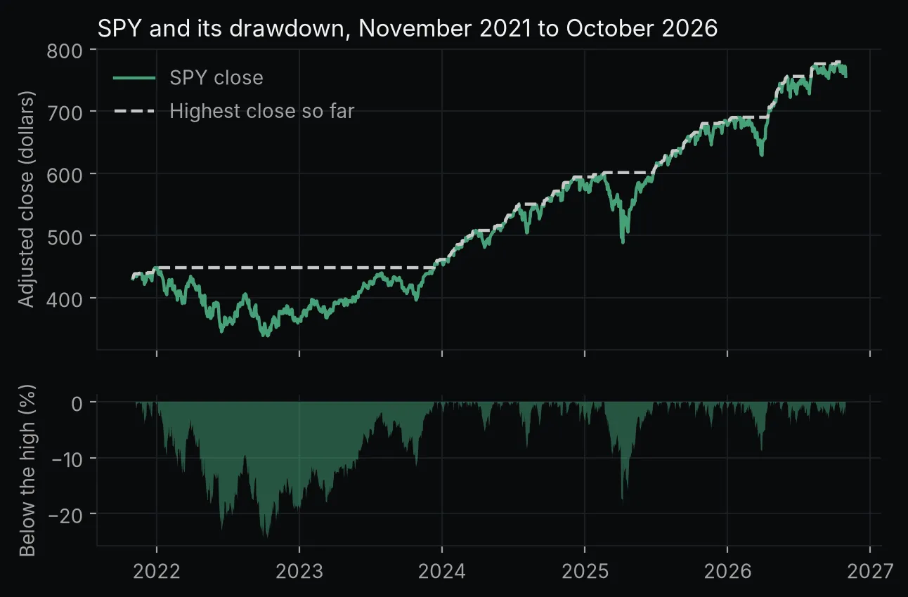 Chart made by this post’s code from Yahoo Finance data (via yfinance, unofficial) through October 30, 2026. Not investment advice.
Wherever the green line touches the dashed one, SPY closed at a new high and the drawdown is zero. The long flat stretch of the dashed line, through 2022 and most of 2023, is the time SPY spent below its old high.
yfinance adjusts Close for dividends and splits by default, so these returns include dividends. The financial analysis tutorial runs the same measures on NVDA against SPY and adds beta, rolling statistics and charts.
2. Risk: value at risk from the same returns
A one-day 95% value at risk (VaR) is the loss exceeded on 5% of days. The historical version reads it straight off past returns:
var_95 = -np.percentile(daily, 5)
worse = (daily < -var_95).sum()
print(f"95% one-day VaR {var_95:.2%}: {worse} of {len(daily)} days lost more")
95% one-day VaR 1.66%: 63 of 1254 days lost moreSPY lost more than 1.66% on 63 of 1,254 days, the 5% the definition promises. A VaR that assumes a bell curve instead comes out too small at the 99% level for SPY, because large moves are more common than a bell curve allows. The quantitative finance tutorial counts those days and adds Sharpe ratios, expected shortfall and a Monte Carlo simulation.
3. Time value of money: npv and irr
Net present value (NPV) is what a series of cash flows is worth today once each one is discounted at a chosen rate. The internal rate of return (IRR) is the rate at which that value comes to zero.
NumPy’s functions for both now live in the numpy-financial package. These are the cash flows its documentation uses for irr: 250,000 out today, then five yearly inflows.
project = [-250_000, 100_000, 150_000, 200_000, 250_000, 300_000]

print(f"NPV at 8%:       {npf.npv(0.08, project):,.2f}")
print(f"Excel-style NPV: {npf.npv(0.08, project) / 1.08:,.2f}")
print(f"IRR:             {npf.irr(project):.6f}")
NPV at 8%: 517,892.29
Excel-style NPV: 479,529.89
IRR: 0.567230At an 8% discount rate the project’s NPV is 517,892.29. npf.npv counts the first cash flow as today, while Excel’s NPV discounts it one period, which divides the result by 1.08 and gives 479,529.89. The IRR, 0.567230 or 56.7%, matches the documentation’s example. The numpy-financial tutorial covers all ten functions, loan schedules and an XIRR for irregular dates.
4. Pricing: a European option in QuantLib
QuantLib prices as of one global evaluation date, so set it first. The option is made up: a six-month European call, the right to buy the stock at 105 (the strike price) on the expiry date only. The stock trades at 100, with 25% volatility, a 4% interest rate and a 1% dividend yield.
today = ql.Date(30, ql.October, 2026)
ql.Settings.instance().evaluationDate = today
dc, cal = ql.Actual365Fixed(), ql.UnitedStates(ql.UnitedStates.NYSE)

process = ql.BlackScholesMertonProcess(
    ql.QuoteHandle(ql.SimpleQuote(100.0)),
    ql.YieldTermStructureHandle(ql.FlatForward(today, 0.01, dc)),
    ql.YieldTermStructureHandle(ql.FlatForward(today, 0.04, dc)),
    ql.BlackVolTermStructureHandle(ql.BlackConstantVol(today, cal, 0.25, dc)),
)
option = ql.VanillaOption(ql.PlainVanillaPayoff(ql.Option.Call, 105.0),
                          ql.EuropeanExercise(ql.Date(30, ql.April, 2027)))
option.setPricingEngine(ql.AnalyticEuropeanEngine(process))
print(f"price {option.NPV():.6f}, delta {option.delta():.6f}")
price 5.537025, delta 0.456551The call is worth 5.537025, and its delta of 0.456551 means it gains about 0.46 for each 1.00 rise in the stock price. The QuantLib tutorial checks this price against a hand-written Black-Scholes formula, then builds a Treasury yield curve from FRED data and prices a bond on it.
5. Valuation: company figures from SEC filings
SEC EDGAR’s CompanyFacts API returns every figure a US company has reported in its filings, free and with no key. SEC’s Accessing EDGAR Data page asks scripts to declare a User-Agent with a name and an email address, and to make at most 10 requests a second. SEC refuses the default User-Agent that requests sends, so put yours in place of the placeholder.
headers = {"User-Agent": "Your Name your.email@example.com"}
url = "https://data.sec.gov/api/xbrl/companyfacts/CIK0000789019.json"  # Microsoft
facts = requests.get(url, headers=headers, timeout=30).json()["facts"]["us-gaap"]

def latest_annual(concept):
    rows = pd.DataFrame(facts[concept]["units"]["USD"])
    rows = rows[(rows["form"] == "10-K") & (rows["fp"] == "FY")]
    rows = rows[(pd.to_datetime(rows["end"]) - pd.to_datetime(rows["start"])).dt.days > 360]
    return rows.sort_values(["end", "filed"]).iloc[-1]

ocf = latest_annual("NetCashProvidedByUsedInOperatingActivities")
capex = latest_annual("PaymentsToAcquirePropertyPlantAndEquipment")
print(f"year ended {ocf['end']}, filing {ocf['accn']}")
print(f"operating cash flow {ocf['val'] / 1e6:,.0f} million")
print(f"capital spending    {capex['val'] / 1e6:,.0f} million")
print(f"free cash flow      {(ocf['val'] - capex['val']) / 1e6:,.0f} million")
year ended 2026-06-30, filing 0001193125-26-323660
operating cash flow 182,935 million
capital spending 115,948 million
free cash flow 66,987 millionMicrosoft’s fiscal 2026 10-K, accession 0001193125-26-323660, reports 182,935 million dollars of operating cash flow and 115,948 million of capital spending, which leaves 66,987 million of free cash flow. The filters matter: each figure also appears as a comparative in later 10-Ks and in other filings, and the duration check drops quarterly rows. The DCF tutorial builds a full discounted cash flow model from inputs like these, with a sensitivity table.
Where can you learn the basics?
If you’re new to Python itself, take a course or read a book before step 1. Our list of the best Python for finance courses and books compares eight, from free ones such as Quantra’s Python for Trading: Basic to Yves Hilpisch’s Python for Finance. Each entry gives its prerequisites and its price as of November 4, 2026.
FAQ
Is Python good for finance?
For work you repeat, yes. The libraries here are free and open source: pandas under the BSD 3-clause license, NumPy under BSD 3-clause plus a few other permissive licenses for bundled code, QuantLib under the modified BSD license. Public data such as SEC filings takes a few lines to pull, as step 5 shows, and every result reruns on new data. For a one-off calculation, a spreadsheet is often quicker.
Which Python libraries are used in finance?
For data, pandas handles tables and time series, NumPy arrays and math, SciPy statistics and matplotlib charts. For finance itself there’s numpy-financial for npv, irr and loan payments, QuantLib for options, bonds and yield curves, and requests for data APIs such as SEC EDGAR. yfinance gets Yahoo Finance prices for free, but it’s unofficial. Its README says it is “not affiliated, endorsed, or vetted by Yahoo, Inc.” and reminds users that Yahoo’s finance API is meant for personal use only.
Is Python better than Excel for finance?
They suit different jobs. Excel is quicker for a one-off model you want to see laid out; Python is better when the same analysis runs again on new data. Watch the conventions when you move between them: the same six cash flows give 517,892.29 with npf.npv and 479,529.89 with Excel’s NPV, because Excel discounts the first cash flow one period.
Can Python predict stock prices?
No code in this guide forecasts prices. It measures what already happened (returns, volatility, drawdown, VaR) and prices instruments from stated inputs. A simulation, like the Monte Carlo in the quant tutorial, shows a range of outcomes under its assumptions, not a forecast.
How long does it take to learn Python for finance?
The courses in our list estimate their material at 6 to 74 hours, from a short portfolio course to a four-course specialization. The examples on this page need only the basics: loading a table, filtering rows and calling a function.
Do you need to know Python before learning Python for finance?
Not for a beginner course. DataCamp’s Finance Fundamentals in Python track and Quantra’s free Python for Trading: Basic both say they have no prerequisites, so you learn the language and the finance together. Others ask for Python first: 365 Data Science’s Python for Finance requires basic familiarity with it, and Lewinson’s Python for Finance Cookbook expects working knowledge of Python, particularly pandas and NumPy.
Where to go next
Pick the step closest to your work and run its tutorial from the top. Each one states the versions and dates it ran on, so your outputs should match until the data changes.